Deep Dive

Understanding the RBLN Runtime and its Workflow

The RBLN Runtime serves as the API for executing compiled models on the RBLN NPU. It provides a direct and simplified interface to the RBLN SDK's core components and directly interacts with the underlying RBLN Driver to manage device execution, memory, and synchronization. This ensures efficient communication between the host application (your code) and the NPU hardware.

Architecture

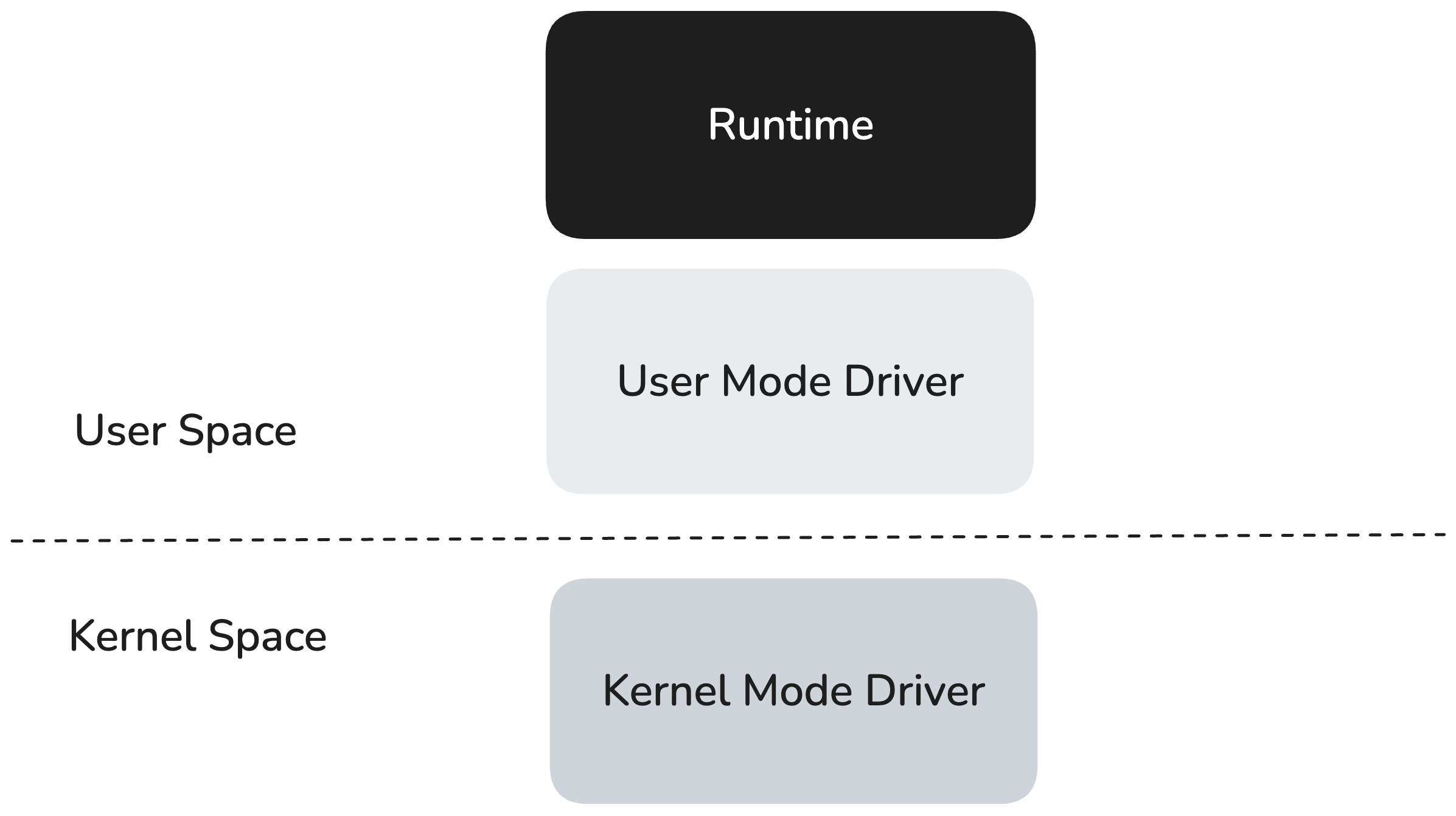
The RBLN runtime operates in the user space, running on top of the user-mode driver (UMD) and utilizing its low-level interface to communicate with the kernel-mode driver (KMD). The KMD runs in the operating system's kernel, where it handles privileged operations such as direct hardware access and scheduling.

Conceptually, the runtime follows a client–server model. The host application acts as the client, making high-level API calls to request tasks such as inference, memory allocation, or synchronization. The NPU acts as the server, executing those tasks. Internally, the runtime translates host requests into low-level commands, encapsulates them in command buffers, and submits them to the RBLN driver, which schedules execution on the NPU.

A Typical RBLN Runtime Workflow

A typical inference workflow is streamlined into three simple steps:

1. Load the compiled file: The .rbln file is loaded into memory.
2. Create the runtime instance: The creation of a rebel.Runtime() object performs the initialization procedures required for inference on the RBLN NPU.
3. Run inference: The module.run() method triggers execution on the NPU.

Here is a simple code example of how to use the RBLN runtime:

import rebel
import torch

# Define input tensor
x = torch.rand(1, 3, 224, 224)

# 1. Load the compiled artifacts from the .rbln file
# 2. Create the runtime instance.
module = rebel.Runtime("simple_conv_bn_relu.rbln", tensor_type="pt")

# 3. Run inference
result = module.run(x)

What’s Inside a .rbln File?

A compiled .rbln file is an optimized container that holds all the necessary data for a neural network to run efficiently on an NPU. It's essentially a pre-packaged, ready-to-run version of your model, designed to minimize latency and maximize performance by eliminating on-the-fly compilation and resource allocation. The file's contents are categorized into three main sections: Model, Metadata, and Profile Info.

1. Model

This section contains the fundamental components of the neural network, all of which have been pre-optimized for efficient execution on the NPU.

• Compiled Graph : This is a directed acyclic graph (DAG) that represents the model's computational flow. For models from frameworks like torch.nn.Module, the original graph is "lowered" into this optimized form. This ensures all operations, including data transfers between the host (CPU) and the NPU, are executed in the correct topological order for maximum efficiency.
• Program Binary : This is the executable machine code specifically compiled for the NPU's instruction set. It contains the low-level operations that the NPU's processor can execute directly, much like an executable file for a traditional CPU.
• Command Stream : An optimized sequence of instructions containing virtual addresses that is consumed by the NPU's command processor.
• Memory & I/O : This component includes precomputed memory addresses and allocation sizes for all tensors—inputs, outputs, and intermediate data. By pre-allocating memory, the .rbln file eliminates the performance bottleneck of dynamic memory management during inference.
• Weights : The model's weights and biases are stored in a highly optimized, pre-compiled format. This allows them to be loaded directly into the NPU's memory without any additional processing or data conversion.

Note

For large language models (LLMs), .rbln files may employ advanced optimizations like weight sharing across different models. This can significantly reduce the file size and memory footprint, making deployment more efficient. As a result, the file's final size and contents may vary depending on these applied optimizations.

2. Metadata

This section contains important structural and compilation information about the model. This data can be inspected programmatically via the RBLNCompiledModel.inspect() API, providing insights into the model's architecture and the specifics of its compilation process.

3. Profile Info

This section contains detailed profiling data, which is essential for performance analysis. This information helps developers understand how the model behaves on the NPU, identifying potential bottlenecks and areas for improvement.

The RBLN Command Structure

The RBLN Runtime uses a structured, low-level command system to orchestrate tasks on the RBLN NPU, similar to how modern graphics APIs manage GPU work.

Command Buffers

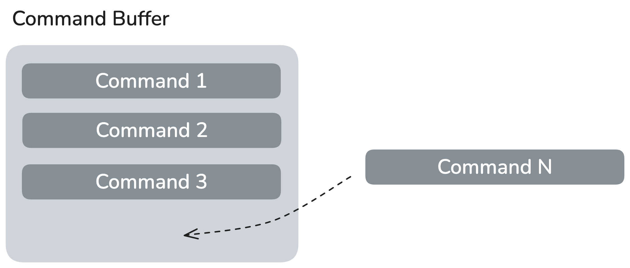
A Command Buffer is the fundamental unit of work submission in the RBLN Runtime. It encapsulates one or more commands that represent a single, atomic task. The RBLN runtime creates these buffers and then encodes them with the precompiled Command Stream and Tensor information stored in the .rbln file.

Lifecycle of an RBLN Command Buffer

1. Creation: During runtime initialization, the runtime creates one or more command buffers. Each buffer represents a logical chunk of the model's execution flow.

2. Encoding: The runtime populates each buffer with specific commands, such as tensor transfers (HDMA), compute kernel dispatches, and synchronization points (barriers) required for a complete inference pass.

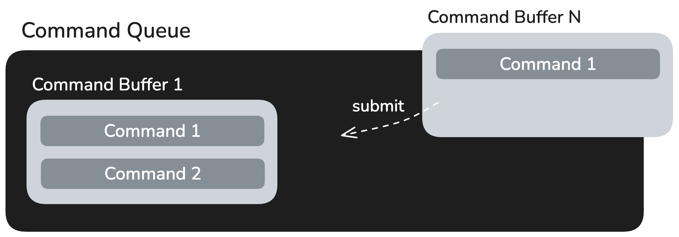
3. Submission: The command buffers are enqueued into the command queue. This action submits the batch of commands to the UMD, which then forwards them to the KMD for scheduling on the NPU.

4. Execution & Completion: The NPU processes the commands asynchronously. Once a command buffer's execution is complete, the driver signals its completion. The runtime can then query the status of the buffer or use a completion handler to trigger subsequent actions.

5. Reuse/Release: The runtime manages the lifecycle of the buffers, either releasing their resources or reusing them for subsequent inference runs to optimize performance.

Runtime Initialization and Execution

Creating a Runtime() Instance

When you create a runtime instance, the .rbln file is loaded and the NPU is prepared for inference. This process involves:

1. Memory Allocation: The runtime allocates necessary device memory based on the precomputed layout specified in the .rbln file.

2. Data Upload: The Command Stream, weights, and other static data are copied from the host to the NPU's memory.

3. Command Buffer Construction & Encoding: As detailed above, the runtime creates command buffers from the uploaded Command Stream and encodes them with specific commands, preparing them for future submission.

4. Device Initialization: Final configuration of the NPU is performed to ensure it is ready for immediate inference execution.

The run() method

Once the runtime is created, the model is fully prepared to perform inference on the RBLN NPU. When runtime execution is triggered, the RBLN NPU runs inference efficiently using the preconfigured Command Buffers. The process is as follows:

1. Input Preparation: Validate the input tensor provided by the user, perform any required transformations, and prepare the output tensor to receive the results.

2. Data Transfer: Transfer the prepared input tensor to the RBLN NPU using external HDMA.

3. Command Submission: The runtime submits the pre-constructed command buffers to the command queue for execution.

4. Execution: Inference on the RBLN NPU is started by the KMD sequentially invoking the command buffers from the command queue.

5. Result Retrieval: Once all command buffers have finished execution, the KMD signals completion. The final command in the buffer is typically an HDMA transfer command to move the results from the NPU's memory back to the prepared output tensor on the host.

Guidelines for Performance Measurement in Rebellions NPU

Methods for Performance Measurement

1. Using time.perf_counter_ns() in Python
   1. Example code:

      import argparse
      import time
      import torch
      import rebel
      
      N_WARMUP = 10
      N_ITERS = 50
      
      @torch.compile(backend="rbln", dynamic=False)
      def matmul(tensor_a: torch.Tensor, tensor_b: torch.Tensor):
         return torch.matmul(tensor_a, tensor_b)
      
      def run(M, N, K):
         tensor_a = torch.randn(M, K, dtype=torch.float16)
         tensor_b = torch.randn(K, N, dtype=torch.float16)
      
         for _ in range(N_WARMUP):
             matmul(tensor_a, tensor_b)
      
         start_time = time.perf_counter_ns()
         for _ in range(N_ITERS):
             matmul(tensor_a, tensor_b)
         # does it need to sync for the accurate benchmark?
         end_time = time.perf_counter_ns()
      
         elapsed_time_ms = (end_time - start_time) / 1e6 / N_ITERS
         tflops = (M * N * (2 * K - 1)) / (elapsed_time_ms * 1e9)
         return elapsed_time_ms, tflops
      
      if __name__ == "__main__":
         parser = argparse.ArgumentParser()
         parser.add_argument("--m", type=int, default=1024)
         parser.add_argument("--n", type=int, default=1024)
         parser.add_argument("--k", type=int, default=1024)
         args = parser.parse_args()
      
         ms, tflops = run(args.m, args.n, args.k)
         print(f"\nelapsed time : {ms} ms / tflops: {tflops} TFLOPs/s")
      

   2. Advantages
      1. It is simple to measure end-to-end time.
   3. Disadvantages
      1. It is difficult to understand details related to execution.
         1. Developers cannot see information such as how much time is consumed on the host execution, or how long host-to-device copy takes.
2. Using get_reports() API
   1. Example and explanation: get_reports()
      1. This shows the execution time in the Runtime graph. For example, the operations like h2d copy executed on host appear as a single op, and the functions executed on device also appear as a single op.
   2. Advantages
      1. This is mainly useful for identifying performance bottlenecks caused by host operations in the overall graph.
   3. Disadvantages
      1. As a tool that measures per-op execution time in the Runtime graph, it has the limitation that it does not account for overheads outside of op execution.
         1. Examples of such overheads include:
            1. Sanity checks (e.g., input shape, dtype) at the Python level before graph execution (typically microseconds).
            2. Unavoidable memcpy due to graph topology before graph execution (can take up to milliseconds).
            3. Terminal output, file I/O, or JSON dump before/after op execution when RUNTIME_TIMER or IODUMP environment variables are set (generally microseconds).
            4. memcpy when allocating new output tensors for the graph after execution (can take up to milliseconds).
3. Using RBLN Profiler
   1. Example and explanation
      1. All individual operations executed on the device are shown as separate ops.
   2. Advantages
      1. Easy to analyze performance bottlenecks by visualizing with Perfetto.
   3. Disadvantages
      1. Profiling overhead may cause differences from the values measured by methods 1 and 2.
      2. Provides information about executed ops, but with limitations in understanding what each op represents.
         1. Users should carefully read the document for interpretation.
      3. Only visualizes profiling information and does not support exporting data (e.g., CSV). As a result, matching results with the get_reports() API can require significant effort.
4. Using torch.profile in vLLM RBLN
   1. Example
   2. Advantages
      1. This provides an overview of overheads occurring throughout vLLM and device execution time at a glance.
   3. Disadvantages
      1. Information about what happens inside the device is not visible.

Precautions for Performance Measurement

1. Perform sufficient warm-up runs before actual measurement.
2. Use repeated executions for measurement, and discuss performance with a representative value (e.g., average).
3. Large deviations in repeated measurements are usually caused by host-side pre-/post-processing. This can be mitigated by providing enough threads with the RBLN_NUM_THREADS environment variable.
4. End-to-end model execution on Rebellions NPU consists of:
   1. Host preprocessing → host-to-device DMA → device compute → device-to-host DMA → host post-processing.
   2. To measure the duration of each step, use the RBLN profiler.
      1. Usage and examples are described in the document.
      2. When running models compiled with torch.compile, execution time includes all of the above processes.
5. Models compiled via torch.compile operate synchronously.

Cautions when using get_reports()

1. Carefully review the get_reports() documentation.
2. To enable get_reports(), set the environment variable RBLN_RUNTIME_TIMER=1.
3. Enabling this option may slightly slow down inference.
4. If get_reports() is used in warm-up code, the warm-up will be included in the statistics and distort results. To avoid this, explicitly call module.flush_reports() after warm-up to clear the data.
5. Consider the following during measurement:
   1. After model load, the first one or two executions may show significantly higher device execution times. Subsequent runs usually stabilize.
   2. Host execution time often fluctuates, showing high variance across runs.