gpt-oss-20b (Data Parallelism)
This page profiles a run divided across several ranks by data parallelism. For basic profiling and trace analysis on a single device, see gpt-oss-20b.
Under data parallelism the model runs in a per-rank worker process rather than in the process that launched the script. One rank is one worker process, using one device. Profiling works the same way in this configuration too: set RBLN_PROFILER=1 and mark the profiling range with vLLM's start_profile() and stop_profile().
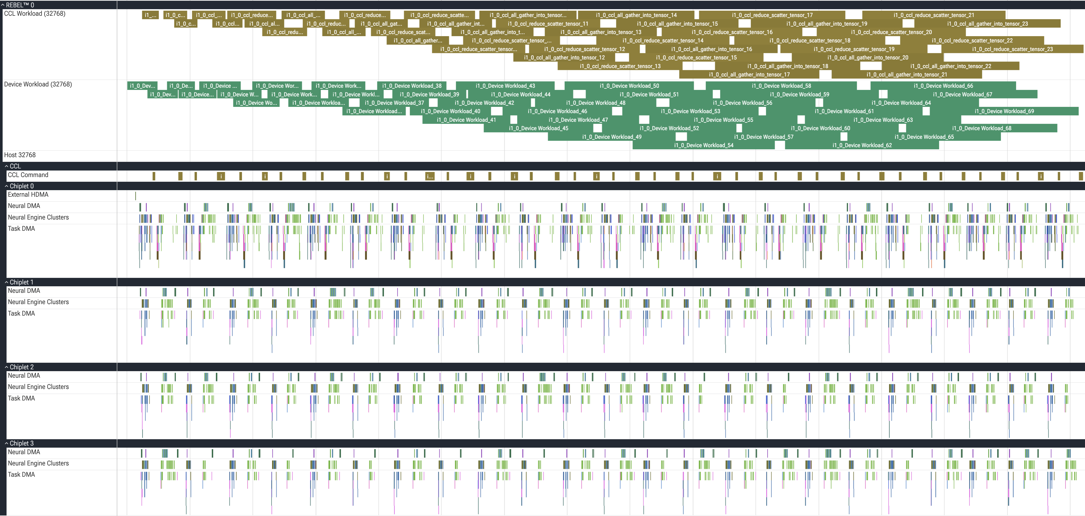
In this case a trace is written per worker, so several ranks produce several traces. The ranks also exchange data through collective communication (CCL), so one run of the model can split into several Device Workload slices with the collectives sitting between them.
Preliminaries
Installation
Install vllm-rbln as described in RBLN vLLM. The example scripts on this page live under examples/ in the vllm-rbln repository, so following the source-code install leaves them in place as well.
Activate RBLN Profiler
Setting RBLN_PROFILER=1 enables the RBLN Profiler.
No additional profiler-specific settings are required for Rebel100™.
Extract Profiled Data with Inference
See data_parallel_offline.py in vllm-rbln for an example of data-parallel execution. To profile a model, keep its execution settings and pass profiler_config when creating the LLM. After warm-up, use start_profile() and stop_profile() to mark the inference range.
The RBLN Profiler runs on the vllm model implementation, and model_impl="vllm" on LLM selects it.
Tip
The code above also enables the PyTorch profiler through profiler_config, which merges the device slices the RBLN Profiler collects into the PyTorch profiler's chrometrace. The per-rank trace merging further below uses those chrometrace files. This merge is supported on Rebel100™ only; it is not available on ATOM™.
This integration needs torch-rbln. Without it, the chrometrace the PyTorch profiler writes holds the PyTorch framework operations alone.
--dp-size sets the data-parallel size and --enable-expert-parallel turns on Expert Parallelism. The example below brings up two ranks.
The run produces as many artifacts as there are ranks. The RBLN Profiler's traces go under a per-rank directory, and the PyTorch profiler's chrometrace goes to the directory named by torch_profiler_dir, one per rank.
Warning
Without start_profile() and stop_profile() marking the profiling range, the trace can be lost. In a multi-process configuration the workers run in their own processes and are torn down when the engine shuts down; any trace data that has not been written to disk by then is lost. stop_profile() returns only after every worker has finished writing, so wrap the profiling range with start_profile() and stop_profile() as vLLM's profiling usage prescribes.
Analysis of Profiled Data from gpt-oss-20b (Data Parallelism) with RBLN Profiler
Collective Communication in a MoE Model
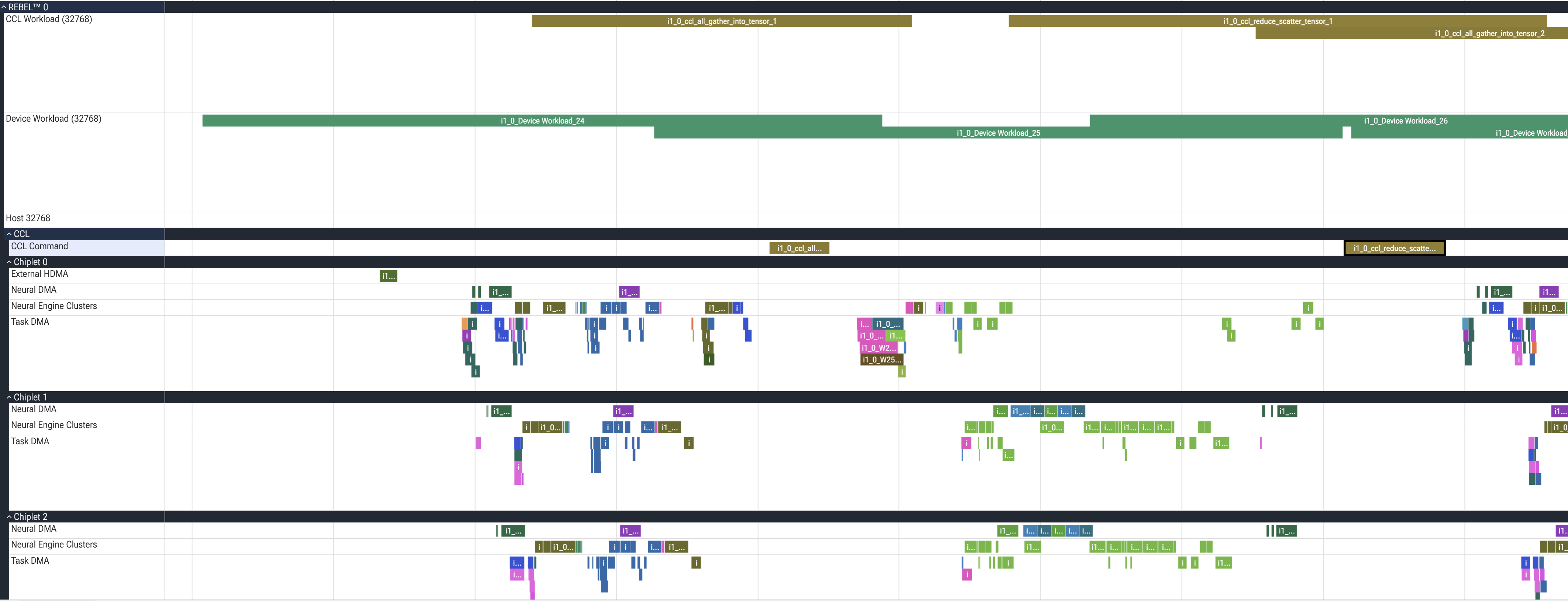
When a model runs across several devices, the ranks exchange data through collective communication (CCL). In a MoE model run with Expert Parallelism, ccl_all_gather_into_tensor and ccl_reduce_scatter_tensor form a pair that repeats layer by layer through the model, and the screenshot zooms in on one such layer.
One layer appears as two Device Workload slices and two collectives. In the screenshot, i1_0_Device Workload_24 → i1_0_ccl_all_gather_into_tensor_1 → i1_0_Device Workload_25 → i1_0_ccl_reduce_scatter_tensor_1 is one layer, and the next one begins at i1_0_Device Workload_26 and i1_0_ccl_all_gather_into_tensor_2. ccl_all_gather_into_tensor collects the tokens, the Device Workload that follows runs the routing and the experts each rank owns, and ccl_reduce_scatter_tensor splits the results back out.
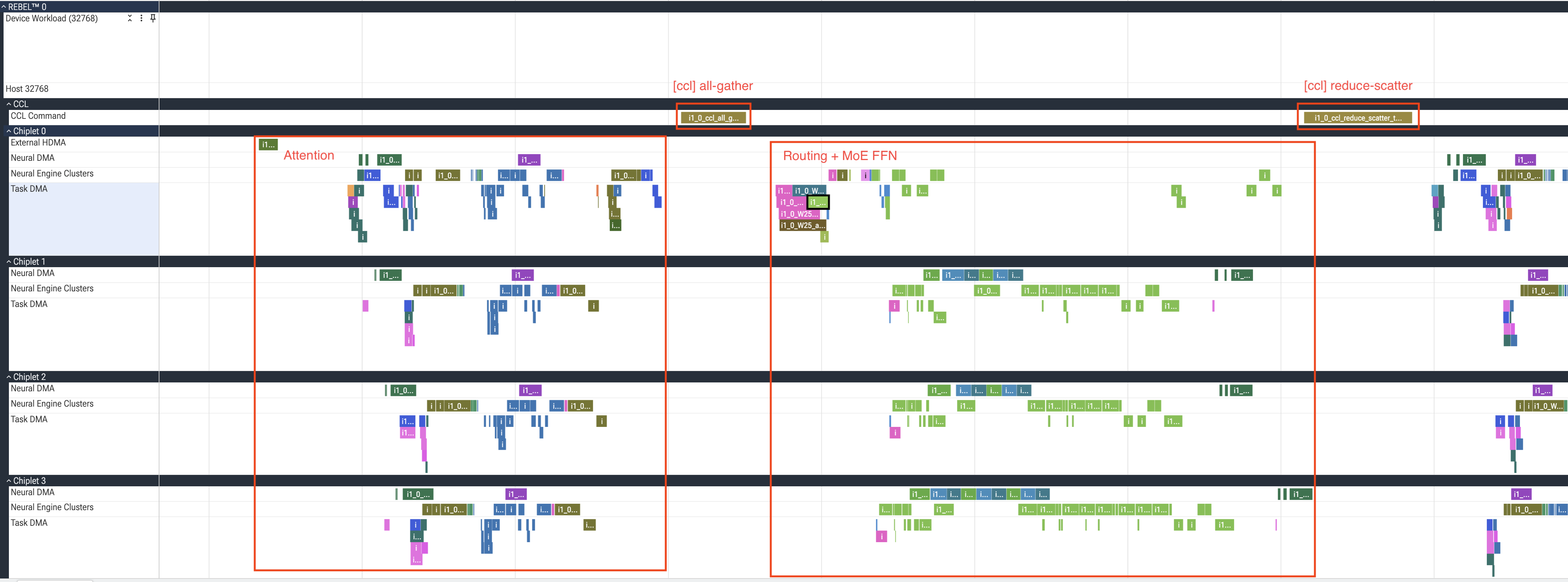
The first Device Workload holds the attention commands, such as input_layernorm and attn_qkv_proj_weight, and the second the routing and expert commands, such as mlp_router_weight and custom_moe_glu_mxfp4. The screenshot marks off those four stages with every chiplet expanded, showing that both the attention and the MoE run split across the four chiplets.
Collective communication appears in the trace at two levels. The CCL Workload track, which sits under Host next to Device Workload, holds one slice per collective covering its whole execution window, and the CCL Command track inside the expanded CCL group holds a slice of the same name covering only the portion in which the command stream runs.
A collective is one operation shared by every rank, so the same slice name appears in each rank's trace. Because the slice covers a rank's whole window for that collective, comparing the same name across the traces shows how long each rank spent waiting for the others.
Per-Rank Trace Merging
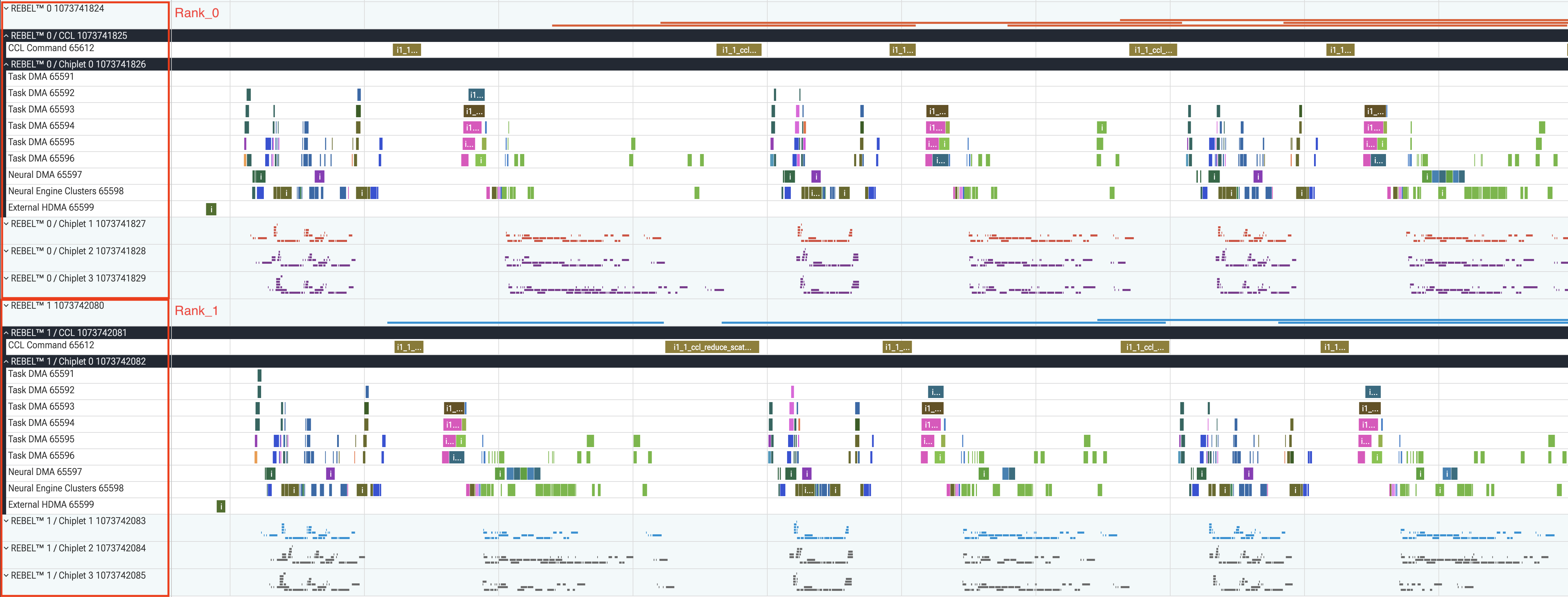
Opening the per-rank traces one at a time makes the relationship between ranks hard to see. The Perfetto UI can merge several chrometrace files onto one timeline. A chrometrace timestamps against the host clock and carries the same reference time, baseTimeNanoseconds, in every file, so files from different ranks land on one time axis.
In the merged view, each rank's tracks stay apart while they share the time axis. In the screenshot, the collectives of the same name finish in the same time window on both ranks.
The procedure, including enabling the plugin, is described in Multiple Traces on One Timeline.
References
- RBLN Profiler
- Analyzing profiler data with Perfetto
- Other profiling examples: Qwen3-1.7B (Text Generation), gpt-oss-20b